Neural network basics, for graphics people
A short reference on the neural-network vocabulary used across the neural texture, neural material and neural appearance posts — MLP, weights and biases, ReLU, forward pass, loss, gradient descent, backpropagation, Adam, latent vectors, feature grids and decoder networks — explained once, concretely, so those posts can link here instead of re-deriving it.
Ben Houston • • 11 min read
This is a reference, not a story. It defines the neural-network vocabulary — MLPs, training, gradient descent, Adam, latent vectors, feature grids and decoder networks — once, carefully, and in plain terms. Nothing here is specific to graphics. If you already know what a multilayer perceptron, Adam and a latent vector are, you don't need this page. (It also underpins the neural-texture compression blog post.)
A model is a function with dials on it#
A model, in this context, is nothing more than a function with adjustable numbers built into it: give it an input, it produces an output, and the exact output for a given input depends on the current values of those numbers. The numbers are the parameters (also called weights when they multiply something, and biases when they just add a constant). Training is the process of adjusting the parameters so the function's output matches some reference you already have. Nothing here requires the function to be a "neural network" specifically — the same words describe fitting a line, a polynomial, or a GGX lobe to measured data. A neural network is just one particular shape of function, chosen because it can represent things a line or a polynomial can't.
The multilayer perceptron (MLP)#
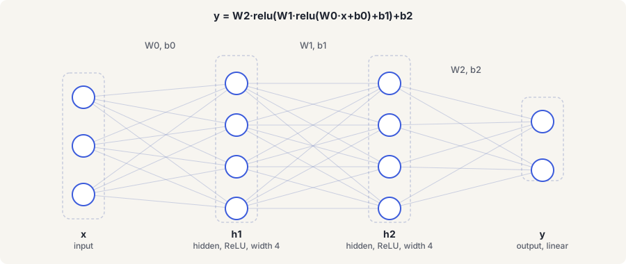
An MLP is a stack of layers, where each layer does the same two things to its input: a weighted sum, then a fixed nonlinear clamp.
is a matrix of weights,
is a vector of biases,
is the input vector, and
is a fixed, non-learned function applied to every element of the result. Stack a few of these and you have an MLP:
Three layers. x is the input, y is the output, h1 and h2 are
hidden layers — "hidden" meaning neither the input nor the output, just
intermediate values nobody outside the function ever looks at directly. The
size of a hidden layer (how many numbers h1 holds) is called its width,
chosen before training and fixed afterward, because it determines the shape of
W0 and W1. Running this function once, input to output, is a forward
pass.
Width and depth (number of layers) are two of the network's hyperparameters, covered more fully below.
That's the entire architecture. An MLP is not more mysterious than this: a short, fixed sequence of matrix-multiply-then-clamp steps.
ReLU, and why the clamp matters#
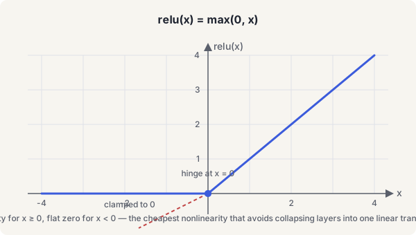
is the most common activation function: identity for positive inputs, zero for negative ones. It's called the rectified linear unit, hence ReLU.
The clamp isn't decoration. Delete it and
,
, which is
— a single matrix, no matter how many layers you stack. Every "deep" network without a nonlinearity between its layers collapses algebraically into one linear transform, and a linear function can't represent anything with a bend or a peak in it. ReLU is the cheapest nonlinearity that avoids that collapse, which is why it's the default choice unless something specific rules it out.
Each ReLU unit behaves like a hinge: it contributes nothing until its input crosses zero, then grows linearly. A layer of many hinges is a piecewise-linear function with that many possible folds, and stacking layers composes those folds into shapes a single layer couldn't reach. More width, more folds, finer approximation — at the cost of more parameters to fit and more work per evaluation.
Loss, gradient descent, and training as fitting#
You've done this before, informally: fit a polynomial through some points, project a function onto spherical harmonics, tune a GGX roughness parameter until a render looks right. All of those are the same activity — a reference you trust, an approximation with free parameters, and an adjustment process that reduces the gap between them.
Concretely, for an MLP:
- Run a forward pass on some inputs you have reference outputs for.
- Compare the network's output to the reference. That comparison, reduced to a single number, is the loss — a plain measure of how wrong the current parameters are. Squared error is the simplest common choice: , where is the network's output and is the reference value.
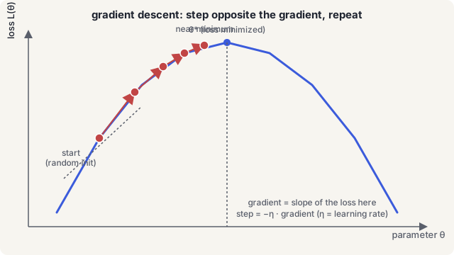
- Compute how the loss would change if each parameter moved a little, in which direction. That's the gradient, , of the loss with respect to the parameters (the collected weights and biases).
- Move every parameter a small step opposite its gradient — downhill on the loss: . The step size is the learning rate.
- Repeat, on a new batch of inputs each time.
One repetition of that loop is a training step or iteration. A group of inputs processed together in one step is a batch, and its size is the batch size. Unlike fitting a polynomial, there's no closed-form solution for an MLP's parameters — you can't just solve for them directly — so training nudges iteratively instead. This iterative process is gradient descent.
Backpropagation, briefly#
Step 3 above — computing the gradient — is done with the chain rule, applied from the output backward through the layers. That algorithm has a name, backpropagation, but the mechanics are ordinary calculus: each layer receives an error signal from the layer after it, uses that signal to compute its own weights' gradients, and passes a modified error signal further back. Two consequences of this matter later. First, a ReLU's derivative is either 1 or 0 (it's linear where it's active, flat where it's clamped), so gradient either passes straight through a unit or stops there completely — a unit whose output is always negative can go permanently silent. Second, computing the backward pass requires the values the forward pass produced at every layer, so running backpropagation costs memory proportional to how many inputs you're processing at once, not just to how many parameters the network has.
Adam#
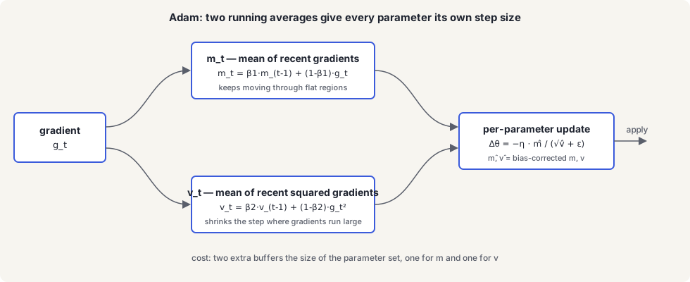
Plain gradient descent takes the same size step for every parameter, which works poorly when some parameters consistently have large gradients and others have small ones. Adam is an optimizer that fixes this by keeping two running averages per parameter: the mean of recent gradients
(so it keeps moving through flat regions instead of stalling) and the mean of recent squared gradients
(so it can shrink the step for parameters whose gradient has been consistently large, and grow it for ones that have been small):
Dividing the first by the square root of the second gives each parameter its own effective learning rate without hand-tuning one per parameter (
is just a small constant that keeps the division from blowing up when
is near zero). The practical cost: Adam needs two extra buffers the same size as your parameter set, one for each running average — a real memory cost when the parameter set includes a multi-megabyte grid of trained values, not just an MLP's weights.
Latent vectors, feature grids, and decoders#
The three graphics posts this page supports all use one more pattern beyond a plain MLP, worth naming precisely because "latent" gets used loosely elsewhere.
A latent vector (or latent code) is a set of numbers that started as free parameters — usually small random values — and were given meaning purely by training, rather than by any predefined encoding a person wrote down. They aren't RGB, they aren't roughness, they aren't anything you could name before training started; whatever structure they end up representing is whatever the optimizer found useful for minimizing the loss. This is different from an ordinary texture channel, where a person decided in advance that this number means roughness.
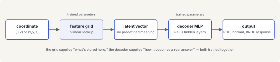
A feature grid is a 2D (or 3D) grid of latent vectors — one small latent vector stored at every grid cell, addressed by a coordinate the same way a texture is addressed by UV. Query it at an arbitrary coordinate and you bilinearly interpolate the latent vectors at the surrounding cells, exactly like sampling a texture, except what you get back isn't a color — it's a latent vector that some other function still has to interpret. A feature grid is itself a set of trained parameters, not a fixed input; it's optimized alongside everything else during training.
A decoder network is the MLP that turns a latent vector (or several, concatenated) into something with an actual meaning again — RGB, a normal, a BRDF response, whatever the task calls for. The pattern across all three posts is: coordinate in, feature grid lookup, MLP decode, meaningful output out. The grid supplies the "what's stored at this location," the decoder supplies the "how do these stored numbers become a real answer," and both are trained together so neither one has to be designed by hand.
Trained parameters vs. everything else#
Worth being precise about one distinction that recurs: a trained parameter is a number training is allowed to change — every weight and bias in the decoder, every latent value in the grid. A hyperparameter is a number a person chooses before training starts and training never touches — layer width, learning rate, batch size, grid resolution, number of training steps. Getting this backward is a common source of confusion: changing a hyperparameter (like grid resolution) changes how many trained parameters exist, but the hyperparameter itself is never something gradient descent adjusts.
Precision: fp32 during training, fp16 often on export#
One practical detail shows up in all three posts and is worth defining once. Training typically keeps every parameter in 32-bit floating point (fp32), because the small updates gradient descent applies at each step need that much precision to accumulate correctly over thousands of iterations. Once training is done, the trained values are often exported at half precision (fp16) — enough precision to reconstruct the result well, at half the storage and bandwidth cost, and (in a WebGPU/WebGL context specifically) because 16-bit float textures are guaranteed hardware-filterable while 32-bit float textures generally aren't without an explicit device feature. That's a statement about what these systems actually do, not a universal law — whether fp16 is "enough" depends on how sensitive the specific output is to rounding, and each post that makes this trade explains why it holds for its own case.
A short glossary#
| Term | Meaning |
|---|---|
| Model | A function with adjustable parameters |
| Parameter / weight / bias | A number training is allowed to change |
| Hyperparameter | A number chosen before training and left fixed |
| MLP | A short stack of weighted-sum-then-clamp layers |
| Hidden layer | A layer that's neither the input nor the output |
| Activation function | The fixed nonlinearity applied after each layer's weighted sum |
| ReLU | , the most common activation function |
| Forward pass | Running the network once, input to output |
| Loss | A single number measuring how wrong the current parameters are |
| Gradient | How the loss would change if each parameter moved slightly |
| Gradient descent | Repeatedly stepping parameters opposite their gradient |
| Learning rate | The size of each gradient-descent step |
| Batch / batch size | A group of inputs processed together in one training step |
| Backpropagation | The chain-rule algorithm that computes gradients layer by layer |
| Adam | An optimizer that gives every parameter its own adaptive step size |
| Latent vector / latent code | Free parameters whose meaning is defined entirely by training |
| Feature grid | A grid of latent vectors, addressed and interpolated like a texture |
| Decoder network | The MLP that turns a latent vector into a meaningful output |
Keep these in hand and the rest of the series should read as engineering, not mathematics you have to take on faith.