Neural Texture Compression in Three.js

A physically-based material is rarely one texture. Base color, normal, roughness, metalness, transmission, emissive: a fully-specified PBR material can be six, eight, ten separate texture maps, each with its own resolution, its own mip chain, its own memory footprint. And those maps are correlated. The edges in a normal map line up with the edges in a roughness map; a metal flake shows up as a coordinated bump in metalness and a highlight in albedo. Ordinary texture compression treats each map as its own unrelated image and throws that correlation away.

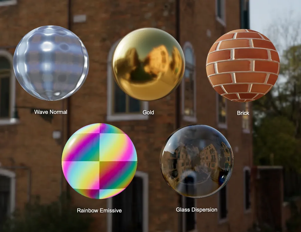
Neural Texture Compression (NTC), the idea behind NVIDIA's 2023 paper of the same name, fits every channel of a material jointly, with one small shared representation, and lets a neural network exploit the correlation ordinary compression ignores. I built an implementation for Three.js: a compact .ntc asset format, a loader, and a decoder that runs directly inside a node material's shader graph. The five materials in the live example each decode from that representation. This post covers what that representation is, how the decoder is implemented, and the performance work that makes it cheap enough to run per-pixel on ordinary hardware.

Some of the terminology below (MLP, ReLU, latent vector) is covered in more depth in a companion primer on neural network basics.

What's actually stored#

An NTC asset is two things: a small multiresolution latent feature grid, and a tiny MLP decoder shared by every channel.

The feature grid is a stack of a few low-resolution textures — three levels in my implementation, each coarser than the last, the same coarse-to-fine idea behind instant-ngp's multiresolution hash encoding. Query it at a UV coordinate, bilinearly filtered and summed across levels, and you get a compact latent vector: a learned feature for that surface point.

The MLP takes that latent vector and decodes it into every channel the material needs, in one forward pass. Each channel gets its own named slice of the output and its own activation function, chosen to match its physical range: sigmoid for bounded [0,1] reflectance-like values (albedo, roughness, transmission), tanh for signed [-1,1] vectors (a tangent-space normal offset), softplus for unbounded non-negative HDR values (emission). A material with ten active channels — say a glass material with albedo, roughness, metalness, transmission, IOR, thickness, attenuation color and distance, and dispersion — trains all ten through that one shared grid and decoder. Those five sample materials run 25.0–31.5KB each for this entire representation: grid plus decoder, every active channel included.

A shared latent representation encodes that correlation once. Independent per-texture compression stores it in every map.

Each asset names its own channels#

Each channel is a small descriptor: a key (roughness, normal, dispersion, ...), a width (1 for a scalar, 2 for a tangent-space offset, 3 for a color), an activation function, and a function that knows how to apply a decoded slice onto a target material's matching property. Loading an asset walks its list of active channels and applies each one in turn.

NTC decodes to whatever named, activated channels this asset was trained against. Adding a new channel type is a new descriptor. The decoder stays the same. I demonstrate the format on a THREE.MeshPhysicalNodeMaterial, the material with the widest channel vocabulary in Three.js. The same asset and evaluator can assign decoded channels onto any other NodeMaterial that exposes matching node properties.

Decoding fast: fp16 storage buffers and mat4-packed evaluation#

None of this is useful if decoding a material costs more than sampling a texture would. Two things make the decoder fast.

Half precision, where the hardware has it. I added f16 support to TSL and to storage buffers at the same time as building this — half, hvec2/3/4, hmat2/3/4 types that behave like their fp32 counterparts everywhere in TSL, compiling to real WGSL f16 on WebGPU with the shader-f16 feature, and falling back to fp32 everywhere else. The decoder's weight matrices live in a real fp16 storage buffer whenever that feature is available:

const weights = instancedArray( matrixCount, 'hmat4' ); // real fp16 storage buffer

Half precision is a well-documented ~2x on every major mobile GPU architecture. Apple's own Metal optimization guidance states that half runs at double rate versus float for vectorized code on Apple GPUs. Arm's GPU Best Practices Guide gives the same ~2x figure for Mali's mediump versus highp across ALU throughput, varying interpolation, and texture sampling. Qualcomm's Adreno Mobile Best Practices docs report the same ~2x for Adreno, down to the hardware detail: Adreno 640 pairs 64-wide FP32 ALUs that need two cycles per wave with 128-wide FP16 ALUs that finish the same wave in one. Three completely different GPU architectures, the same number, for the same underlying reason — halving a value's width roughly doubles how many of it a fixed-width ALU can push through per cycle, and halves the memory traffic for every weight the decoder reads.

Packed mat4 × vec4 evaluation. Each linear layer's weights are packed into mat4 blocks — four output neurons by four input features per block — and evaluated with a single mat4 * vec4 multiply. Four independent dot(vec4, vec4) calls, one per output neuron, do the same arithmetic as four separate instructions; the packed multiply issues effectively one. That's an architectural ceiling of up to 4x fewer instructions for the multiply. The realized speedup depends on register pressure, occupancy, and memory bandwidth, so I'd treat 4x as a ceiling this technique can approach. Directionally it is the same trick as the fp16 win: fewer, wider operations.

Between the two, decoding one texel costs on the order of 500 FLOPs, cheap enough on an average consumer mobile GPU.

Small grids, small networks#

The decoder network is small: two hidden layers of 8 nodes each. That's smaller than the network NVIDIA's paper uses. I chose it because in my experiments, the resolution and level count of the multiresolution latent feature grid mattered more to reconstruction quality than the size or depth of the MLP.

A bigger, deeper network spends its extra capacity re-deriving spatial detail the grid should already be carrying; a richer grid gives the network detail to work with in the first place, and a small network is enough to decode it. Scaling the grid rather than the network is also the cheaper trade at inference time. Grid lookups are hardware-filtered texture samples, cheap, while every extra MLP layer is more matrix-vector work per texel.

What's not here yet#

Two things worth flagging:

No mip pyramid yet. The current implementation samples the latent grid at a single resolution regardless of view distance, so there's no built-in mechanism for reducing aliasing on a material viewed from far away or at a glancing angle, the same problem ordinary textures solve with a mipmap chain. It's on the list; multiresolution NTC in the literature already establishes how to do this, it's a matter of implementing it.

Where the assets come from. Every asset here was trained. Fitting a grid and decoder to a set of source channels is itself a nontrivial GPU training problem, with its own optimizer, quantization, and convergence questions. That's a substantial enough topic for its own writeup. I'll cover the training side in a follow-up.

PR: (link pending)